In this paper we attempt to find a computationally efficient way to numerically simulate networks with nonlinear stochastic dynamics. With this I mean a continuous dynamical model where the differential equation for each variable depends nonlinearly on some or all variables of the system and has additive noise. If $x$ is a vector with all variables and $\eta$ is a random vector of the same size as $x$ with some unspecified distribution, the dynamics can be compactly described as \(\frac{d x}{dt}=f(x,t)+\eta\)
The challenge lies in the nonlinearity combined with stochasticity. Were only one of them to be present, the problem would be simple. A deterministic nonlinear problem can be straightforwardly be integrated with an ODE package, while a linear stochastic system can be reduced to a system of ODEs for the moments of the probability distribution function (PDF). A full solution would require a Monte Carlo algorithm to simulate a sufficient number of paths to allow us to estimate the PDF of $x$ at each time point. For networks with many nodes we are haunted by the curse of dimensionality, as the volume needed to be sampled increases exponentially and so do the number of simulated paths required to get a good approximation of the distribution at later time points. In systems where there is a well defined mode around which most of the probability mass is concentrated we should be able to derive an analytic approximation which is more tractable. This is exactly what we try to do in the paper.
In such cases, we can try to approximate the exact PDF with a multivariate Gaussian distribution, which is the most natural choice under the principle of maximum entropy if we are only interested in the average and covariance matrix. In the cases in which this algorithm is applicable higher order moments contain little information about the PDF of interest, and for most applications we care only about these two moments anyway. Using the Kullback-Leibler divergence as an objective function measuring the quality of the approximation, we can find the parameters which minimize the divergence and obtain the desired approximation.
Surprisingly, these equations depend only on gaussian expectation values, and if we know how to calculate them we are done. In most of the cases, it is hard to compute this for a nonlinear function, so we must taylor expand. Taking a first order expansion results in a linear approximation, which can already be found literature. Higher order expansions provide better approximations, mostly because of the appearance of mixed terms where the average is multiplied by the covariance matrix. These terms mean that the fluctuations affect the mean trajectory unlike in the linear case, where mean and covariance evolve independently. This interaction often leads to a dampening of the dynamics, as you would intuitively expect, because trajectories get out of sync and start cancelling out, dampening the average value. You can see this in the plots comparing the approximations with Monte Carlo runs.
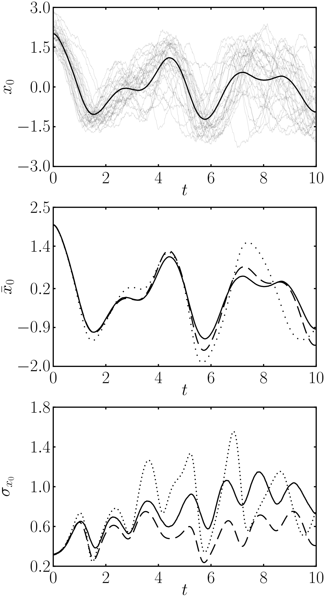
First panel, monte carlo simulation. Second panel, averages for monte carlo (solid), linear approximation (dotted) and our method (dashed). Third panel, standard deviation for all methods.
The final equations are similar to the prediction step for the extended Kalman filter, which is often applied in filtering problems. In this context a single trajectory of the system is observed by some noisy channel, and the goal is to estimate that particular trajectory from the observations. In our case, the aim is to reconstruct the PDF (or some significant statistics) for the whole population. Perhaps this similarity is not surprising given the gaussian approximation. I would be interested in seeing how other methods from the filtering/smoothing community could be adapted to use in our context as well, such as the unscented Kalman filter, or the particle filter. It will not be straightforward though, because in multimodal distributions the average and other moments depend strongly on points in a very wide region in phase space, while in the case of filtering we can always focus on a narrow region around the observation.
In the context of biochemical reaction networks, there was some initial confusion regarding the range of applicability of this method. For discrete systems, a master equation approach makes more sense while many researchers think for continuous systems rate equations are a good enough description. As evidenced by the simulations, in many cases fluctuations directly affect the average values, leading to significant deviations from the deterministic values.