Let’s say you have a bunch of time series data with some noise on top and want to get a reasonably clean signal out of that. Intuition tells us the easiest way to get out of this situation is to smooth out the noise in some way. Which is why the problem of recovering a signal from a set of time series data is called smoothing if we have data from all time points available to work with. This means we know $x_t$ for all $t\in[0,T]$. If we only know $x_t$ up to the current time point $t_n$, i.e. $t\in[0,t_n]$, then the problem is called filtering; and if we only have data for $t\in[0,t_{n-1}]$ the problem is called prediction. These three problems are closely related and the algorithms I’ll discuss are applicable to all problems with minor modifications. I’ll approach the problem from the smoothing perspective since that is what I need for my own research.
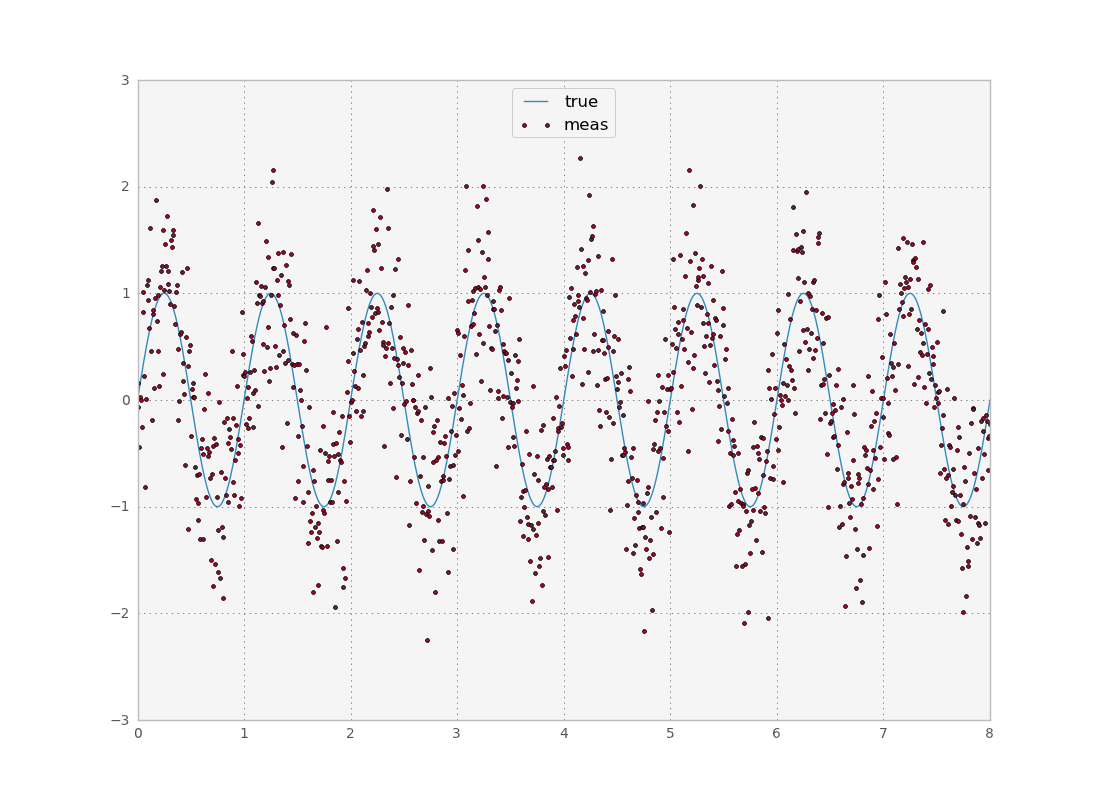
Let’s start by generating a signal $s$ and a measurement $y$ with random noise $n$:
if __name__ == '__main__':
	npts = 1024
	end = 8
	dt = end/float(npts)
	nyf = 0.5/dt
	sigma = 0.5
	x = np.linspace(0,end,npts)
	n = np.random.normal(scale = sigma, size=(npts))
	s = np.sin(2*np.pi*x)
	y = s + n
	plt.plot(x,s)
	plt.plot(x,y,ls='none',marker='.')
The easiest thing one could do would be to average out the points within a small interval. This is called a moving average. It works OK if you have a lot of data and little noise, but that’s not fun at all. If you wanted to be a bit more clever, you could expand the window to a larger time interval to use more information, but weigh the points which are further away from the current time point less, since it might be the case that they have different values not because of noise but because the signal is different at that time. Let’s call the signal $s$ and its estimate $\hat{s}$. Then the exponential moving average is
This window only uses points from the past, with a weight that decays exponentially: $(1-r)^k$ if they are $k$ steps away. A better thing to do would be to also use points from the future. This suggests using a weight function centered around the current point which decays as we step further along. A general formula for this would be:
where the weighing function $f$ is convolved with the measurement inside a window of size $N$. This operation is called a filter because it filters out some frequencies in the signal, while leaving others intact (we’ll explore the frequency spectrum in a bit). Note filters also solve the problem I described as filtering with some lag because we only need the points up to time $t+N$ to know the answer for $t$.
The function $f$ function is known in physics as a Green function or in the signal processing literature as an Impulse response function. A common choice which also decays exponentially is a gaussian function. Let’s try:
def testGauss(x, y, s, npts):
	b = gaussian(39, 10)
	ga = filters.convolve1d(y, b/b.sum())
	plt.plot(x, ga)
	print "gaerr", ssqe(ga, s, npts)
	return ga
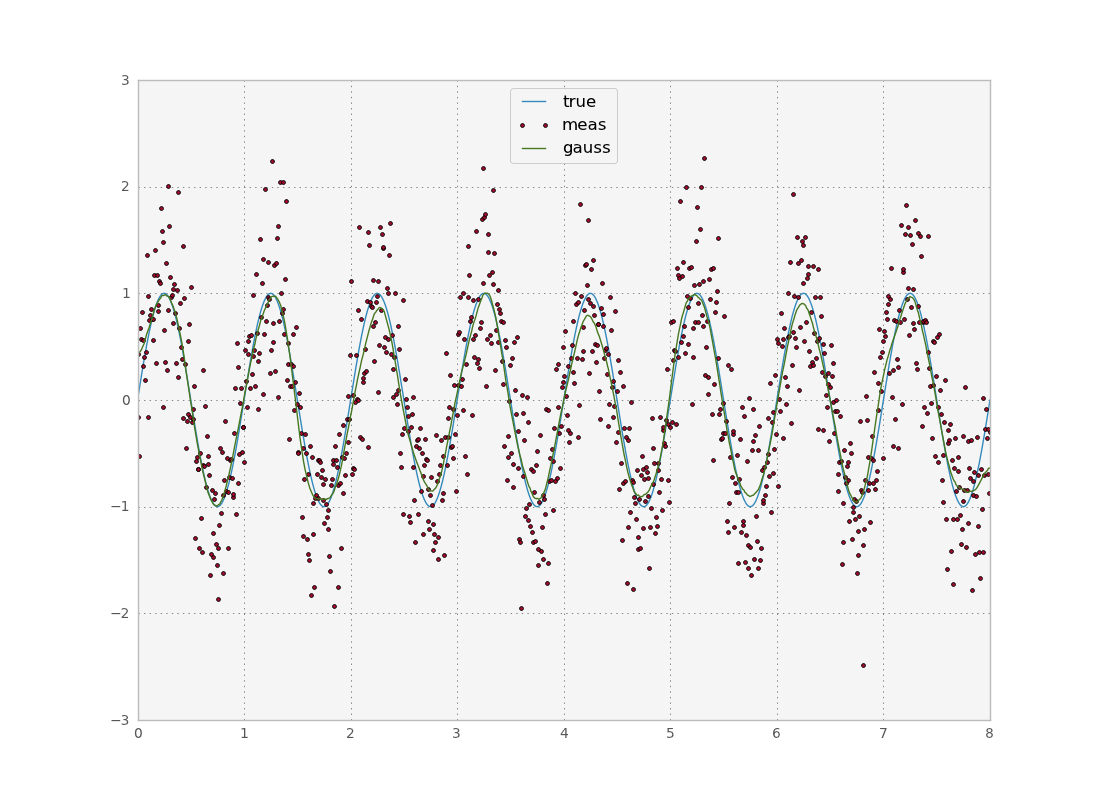
We have an error of 0.0036. Not bad. The gaussian window we used only had $N=39$ values even though theoretically the gaussian extends into infinity. Since it decays exponentially however, we get good results if we cut it off after some values. We can also implement filters with an infinite support. Historically, these kinds of filters were implemented in an analogue circuit, where there is feedback and thus all points interact with each other (explaining the infinite support). The impulse response function described the behavior of the system when presented with a single impulse (hence the name). We can then describe the behavior of the system under any input $y$ by the convolution of the input with the IRF.
Nowadays a distinction is drawn between finite and infinite impulse response filters. The finite filters are pretty easy to use, since all you need to do is a discrete convolution with the signal. The infinite response filters usually have better quality, but are harder to implement on a computer. To implement them, we must use the laplace transform to determine the transfer function
Each filter is uniquely determined by its coefficients $a$ and $b$. Note that a FIR filter has only $a_j=0$ for all $j>0$ so this representation is universal. To try this out, I picked the butterworth filter:
def testButterworth(nyf, x, y, s, npts):
	b, a = butter(4, 1.5/nyf)
	fl = filtfilt(b, a, y)
	plt.plot(x,fl)
	print "flerr", ssqe(fl, s, npts)
	return fl
For our simple test data, the error is approximately the same as in the gaussian window case. Note that the filter design function in scipy takes the cuttoff frequency divided by the nyquist rate. Also note the use of the filtfilt, which applies the filter once forward and once backward to eliminate the lag due to the fact that the convolution needs to ‘buffer’ some initial points at the beginning. This way the forward lag is compensated by the backwards lag (some automatic padding is applied to get an estimate for all $t$). I could have used this function for the gaussian filter as well, passing [1.0] for the $a$ parameter.
To understand how these filters differ it is useful to look at their frequency response. In fourier space, convolution becomes a multiplication, and we can understand what a filter does by looking at which frequencies it lets pass through. An ideal filter should let a range of frequencies pass through and completely cancel the others. However usually there is some regime where there is some attenuation, the width of which depends on the filter’s order. You don’t want a filter with too high an order though, because instabilities occur near the cutoff frequency.
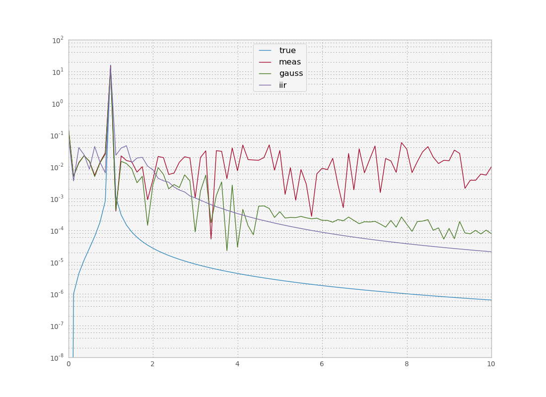
In our simple case we only want to let one frequency pass through and cut off all the others. We see that the signal frequency is a sharp peak and then the power of all other frequencies dies out quickly. On the other hand the measured noisy signal has some constant power for all frequencies (this is where the term white noise for a gaussian comes from, because all frequencies have equal power). Our filters essentially filter out all frequencies above a certain frequency. They are called low pass filters. We could also design high pass or band pass filters, if the frequency were in some other region of the spectrum. In all cases, we have to know beforehand approximately the frequency of the signal we are looking for. If we don’t know that we have to get more sophisticated.
Full code below (with some stuff to be covered in the next post too):
'''
Created on Mar 16, 2013

@author: tiago
'''

import numpy as np
from scipy.interpolate import UnivariateSpline
from scipy.signal import wiener, filtfilt, butter, gaussian, freqz
from scipy.ndimage import filters
import scipy.optimize as op
import matplotlib.pyplot as plt

def ssqe(sm, s, npts):
	return np.sqrt(np.sum(np.power(s-sm,2)))/npts

def testGauss(x, y, s, npts):
	b = gaussian(39, 10)
	#ga = filtfilt(b/b.sum(), [1.0], y)
	ga = filters.convolve1d(y, b/b.sum())
	plt.plot(x, ga)
	print "gaerr", ssqe(ga, s, npts)
	return ga

def testButterworth(nyf, x, y, s, npts):
	b, a = butter(4, 1.5/nyf)
	fl = filtfilt(b, a, y)
	plt.plot(x,fl)
	print "flerr", ssqe(fl, s, npts)
	return fl

def testWiener(x, y, s, npts):
	wi = wiener(y, mysize=29, noise=0.5)
	plt.plot(x,wi)
	print "wieerr", ssqe(wi, s, npts)
	return wi

def testSpline(x, y, s, npts):
	sp = UnivariateSpline(x, y, s=240)
	plt.plot(x,sp(x))
	print "splerr", ssqe(sp(x), s, npts)
	return sp(x)

def plotPowerSpectrum(y, w):
	ft = np.fft.rfft(y)
	ps = np.real(ft*np.conj(ft))*np.square(dt)
	plt.plot(w, ps)

if __name__ == '__main__':
	npts = 1024
	end = 8
	dt = end/float(npts)
	nyf = 0.5/dt
	sigma = 0.5
	x = np.linspace(0,end,npts)
	r = np.random.normal(scale = sigma, size=(npts))
	s = np.sin(2*np.pi*x)#+np.sin(4*2*np.pi*x)
	y = s + r
	plt.plot(x,s)
	plt.plot(x,y,ls='none',marker='.')
	ga = testGauss(x, y, s, npts)
	fl = testButterworth(nyf, x, y, s, npts)
	wi = testWiener(x, y, s, npts)
	sp = testSpline(x, y, s, npts)
	plt.legend(['true','meas','gauss','iir','wie','spl'], loc='upper center')
	plt.savefig("signalvsnoise.png")
	plt.clf()
	w = np.fft.fftfreq(npts, d=dt)
	w = np.abs(w[:npts/2+1]) #only freqs for real fft
	plotPowerSpectrum(s, w)
	plotPowerSpectrum(y, w)
	plotPowerSpectrum(ga, w)
	plotPowerSpectrum(fl, w)
	plotPowerSpectrum(wi, w)
	plotPowerSpectrum(sp, w)
	plt.yscale('log')
	plt.xlim([0,10])
	plt.ylim([1E-8,None])
	plt.legend(['true','meas','gauss','iir','wie','spl'], loc='upper center')
	plt.savefig("spectra.png")