If we have a mathematical model for the system in study, we can use that information to dramatically improve the quality of our prediction. Like in the previous filtering methods, we are taking advantage of the fact that to estimate the system state at some time $t$ we can use not only the information available at that time but also the information from the past (and the future if smoothing). But model free methods tend to want to reduce large deviations from one point in time to the next, while we may actually expect that at some specific time point the system does jump drastically in value. Adding in the model allows us to take that into account.
Let’s start by looking at the Kalman Filter, which is the optimal estimator for linear and gaussian systems. Let us define such a system first in the discrete case:
\[x_{n+1} = Ax_{n}+\xi \\ y_{n+1} = Bx_{n+1}+\zeta\]The stochastic process in $x$ is the underlying process we want to follow. Not only is the process in $x$ a brownian process (additive white noise denoted by $\xi$), we are unable to observe it directly. The observation is denoted by $y$ and is a function of $x$ corrupted by (again) additive white noise $\zeta$. The gaussian assumption is often a reasonable approximation to the problem’s noise statistics because the timescale of whichever microscopic process produces randomness is usually much smaller than the one of the actual dynamics, allowing the central limit theorem to kick in.
In this case, the Kalman Filter is the optimal estimator for the system in the sense that no other estimator can have a smaller mean square error. I won’t reproduce the algorithm here, because we’ll discuss the nonlinear version of it later; you can easily find it on
wikipedia if you really want to. Because there are no free lunches, it turns out this class of systems is quite limited. Most interesting systems do not have linear dynamics, so we need to find an estimator for such nonlinear systems:
\[x_{n+1} = f(x_{n})+\xi \\ y_{n+1} = g(x_{n+1})+\zeta\]The obvious thing to try would be to extend the kalman filter by linearizing the systems. This is done by replacing the functions f and g by their first order taylor expansions around the current value. This results in a set of linear equations like the ones we had previously where $A$ is the jacobian of $f$ and $B$ the jacobian of $g$. Let’s look at the equations for the extended kalman filter for the case of continuous time, where we assume we also have a continuous flow of information (in real cases, and in our tests below, we actually have a continuous time system with discrete measurements. In this case, you simply integrate the part of the equations that do not relate to the measurement up to the measurement time and then do the filter update as normal).
\[\begin{align} \frac{d\hat{\mathbf{x}}}{dt} &= f(\hat{\mathbf{x}}(t))+\mathbf{K}(t)\Bigl(\mathbf{y}(t)-g\bigl(\mathbf{x}(t)\bigr)\Bigr) \\ \frac{d\mathbf{P}}{dt} &= \mathbf{F}(t)\mathbf{P}(t)+\mathbf{P}(t)\mathbf{F}(t)^{\top}-\mathbf{K}(t)\mathbf{G}(t)\mathbf{P}(t)+\mathbf{Q}(t) \\ \mathbf{K}(t) &= \mathbf{P}(t)\mathbf{H}(t)^{\top}\mathbf{R}(t)^{-1} \\ \mathbf{F}(t) &= \left . \frac{\partial f}{\partial \mathbf{x} } \right \vert _{\hat{\mathbf{x}}(t)}\\ \mathbf{G}(t) &= \left . \frac{\partial g}{\partial \mathbf{x} } \right \vert _{\hat{\mathbf{x}}(t)} \end{align}\]I adapted these from wikipedia, simplified for clarity.
Let us look at what the equations mean.
The first equation is the evolution of the system state mean.
The mean value is evolved with the nonlinear function and then corrected by the value of the observation we made weighed by some factor $K$.
Already here we see what could go horribly wrong: for a nonlinear system $<f(x)>\neq f(
It turns out this works quite well if we have a lot of measurements and the fluctuations are small because for small time steps the function which represents the dynamics will be well represented by a linear approximation. Then we are ‘following’ the system very closely and therefore we don’t really care about its nonlinear nature. However, if the observation points are too widely spaced apart or there are large fluctuations then in that long time interval the system might evolve into a number of distinct regions of phase space because of the nonlinearity and the Kalman Filter’s Gaussian distribution no longer accurately models our information about the system. What are ‘large’ fluctuations however?
In the picture below I ran a stochastic simulation for the case of a bistable switch, shown in the inset. In this case, there is an unstable fixed point at x=0.5 and two stable fixed points at 0 and 1. Any small deviation around 0.5 will push the system to the closest stable point. Now, if you have a stochastic system and you start off at the point x=0.5, any small perturbation will send you flying off to either the left or right stable points. You can see that happening to the trajectories in the figure below.
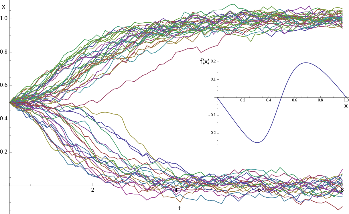
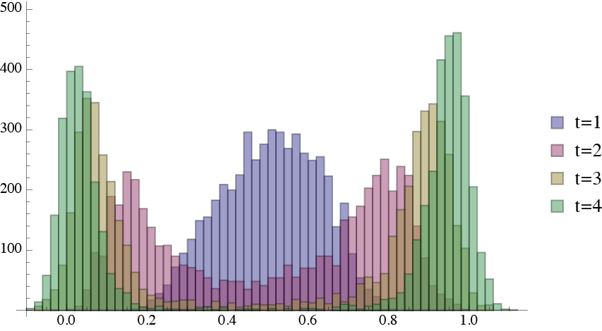
If the noise source in the system is a white noise, then you get a 50% probability of going to either side, which means that the probability distribution starts off gaussian but then splits into two: a bimodal distribution.
Now imagine we are tracking a single trajectory of this system with the Kalman filter. If we have a small time step and some reasonable noise level, we can follow the system trajectory to either one of the stable system states. But if the time step is too coarse, the Kalman filter would be trying to represent a bimodal probability distribution by a gaussian, which would give some terrible result. In this case, even if the time step would be too coarse we would eventually figure out where we are, because we would accumulate enough statistics to know whether we ended up in one side or the other, and then locally you can represent that part of the probability distribution by a gaussian. Additionally, if the noise would be of order one, it would be hard to localize the system in either one or the other side, but this would affect any method, linear or not.
Keeping these caveats in mind, let’s test out the Kalman filter. Our python implementation assumes the function g is the identity, which simplifies the code somewhat. The system being simulated is the van der pol oscillator. To calculate the derivatives I use an algorithmic differentiation package, which calculates the derivatives of any function implemented in code just by looking at its computational graph (the set of elementary operations which make up the function and their relations). This is still like magic to me even today: you can take a function which integrates an ode and derivate it with respect to the input parameters. This is akin to calculating a path derivative, which is something you can’t even do analytically for most systems! In this case, the usage is simpler because we only need to take the derivative of the function being integrated.
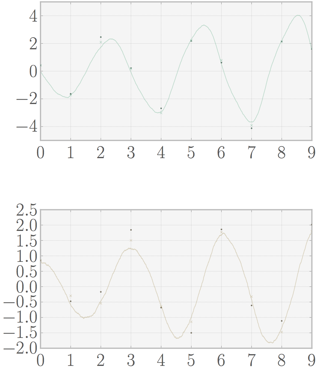
If we use only one oscillator with a slightly stochastic system (sigma 0.01) and reasonable measurement noise (sigma 0.1) we have a really good estimate (mse 0.086). You can look at the plot below (dots are measurements, crosses are predictions).
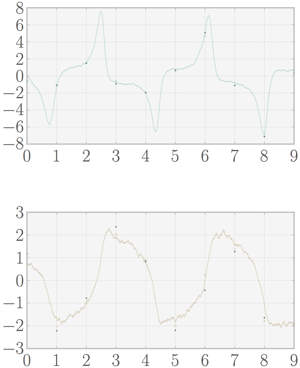
If we tune up the nonlinearity parameter in the van der pol equations the error increases (mse 0.135) as you can see below. However if we’d increase the number of data points the quality of the prediction would increase, and we’d still have a pretty good estimate of the system (because the linearization assumption is a better approximation for small time steps as we discussed above).
As a final remark, I should mention that the filter equations need as input the noise strength of both stochastic processes. In the test cases I showed here I plugged in the correct fluctuation values (the same as used for the simulations), while in a real system we do not know the true value which would be another source of error. Yet, in most cases a reasonably good estimate can be made for these parameters such that the basic properties we discussed here are still valid.