In one of my recent projects I was interested in learning a regression for a quite complicated data set (I will detail the model in a later post, for now suffice to say it is a high dimensional time series). The goal is to have a model which given an input time series and an initial condition is able to predict the output at subsequent times. One good tool to tackle this problem is the recurrent neural network. Let’s look at how it works and how to implement it easily in python using the excellent theano library.
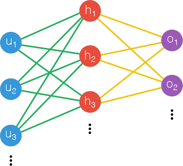
A simple feed forward neural network consists of several layers of neurons: units which sum up the input from the previous layer and a constant bias and pass it through a nonlinear function (usually a sigmoid). Neural networks of this kind are known to be universal function approximators (i.e. for an arbitrary number of layers and/or neurons you can approximate any function sufficiently well). This means that when you don’t have an explicit probabilistic model for your data but just want to find a nonparametric model for the input output relation a neural network is (in theory, not necessarily in practice) a great choice.
In vector notation, the output of the middle layer can be written as is $h = g(W_{hu}.u + b_h)$ with W the weight matrix, b the bias, u the input and g the sigmoid function. If we want to create a deep network we’d stack additional middle layers with the output of one the input of the next. Finally the output will be $o = g(W_{oh}.u + b_o)$.
The Theano library for python is an ideal framework to implement neural networks in, even though it is more general than that. Theano allows us to define the mathematical expressions we will need to compute and then compile them directly to machine code (cpu or gpu), which makes it great for scientific computation: you can develop quickly thanks to python and not sacrifice performance (there are some downsides: it’s reasonably hard to debug and the code can get confusing at times).
Before proceeding, take a look at the tutorials. There is even a deep learning tutorial which has a sample feedforward network implementation which you can take and use to quickly get started with feedforward neural nets. The network class adds each layer’s output to the next one’s input, building up the computational graph for the network. I’d recommend you take a look at the tutorial to learn more about how to train the neural network using mini batch stochastic gradient descent, because we’ll use that later on.
In many cases (time series analysis etc..) you’ll have a very high dimensional data set which you need to feed to your network. You could use a simple feedforward neural network and feed all dimensions as inputs. But this comes with downsides: first, the dimensionality of your first layer will be huge, leading to more parameters to learn; second, if the data really is dynamic it could be the case that inputs will have different dimensionality and there is no elegant way to handle that. They key insight is that because there is structure in the data, a model with memory will be able to build up a ‘compressed’ picture of the data as each data point is fed into it.
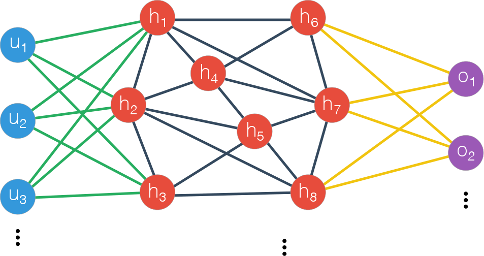
A recurrent neural network is precisely such a model with memory: at each time step it is fed some input plus the state of its hidden units in the previous time step. I’ve sketched the recurrent network below:
Mathematically, the hidden layer now has an output described by: $h^{t} = g(W_{hh}.h^{t-1} + W_{uh}.u^t + b_{h})$. In the image the two weight matrices are distinguished by the different colors in the connections: the hidden to hidden connections are dark blue while the input to hidden are green. Note that the network doesn’t have to be fully connected, we could very well use sparse W matrices (and can impose that as a training constraint by adding $L_1$ regularization).
There is a very complete example on how to use recurrent neural networks in theano here, but it’s quite advanced and so I’ve implemented a much simpler recurrent network based on that code to get a feel for this model (my full code here). To start with we define all the different parameter variables (i.e. the W and b) as shared variables and define some other symbolic variables as well.
'''define random state and activation function'''
rng = np.random.RandomState(1234)
self.activ = T.nnet.sigmoid

'''define symbolic variables'''
lr = T.scalar()
u = T.matrix()
t = T.scalar()

'''define shared variables'''
W_uh = np.asarray(rng.normal(size=(nin, n_hidden), scale= .01, loc = .0), dtype = theano.config.floatX)
W_hh = np.asarray(rng.normal(size=(n_hidden, n_hidden), scale=.01, loc = .0), dtype = theano.config.floatX)
W_hy = np.asarray(rng.normal(size=(n_hidden, nout), scale =.01, loc=0.0), dtype = theano.config.floatX)
b_hh = np.zeros((n_hidden,), dtype=theano.config.floatX)
b_hy = np.zeros((nout,), dtype=theano.config.floatX)

W_uh = theano.shared(W_uh, 'W_uh')
W_hh = theano.shared(W_hh, 'W_hh')
W_hy = theano.shared(W_hy, 'W_hy')
b_hh = theano.shared(b_hh, 'b_hh')
b_hy = theano.shared(b_hy, 'b_hy')
To define the network dynamics we use the scan operation, which allows us to define loops. We give it an initial state and an input sequence ($h_0$ and $u$ in this case) and provide the code that should be run at each step:
'''network dynamics'''
h, _ = theano.scan(self.recurrent_fn, sequences = u,
                   outputs_info = [h0_tm1],
                   non_sequences = [W_hh, W_uh, W_hy, b_hh])

'''network output'''
y = T.dot(h[-1], W_hy) + b_hy

'''recurrent step'''
def recurrent_fn(self, u_t, h_tm1, W_hh, W_uh, W_hy, b_hh):
    h_t = self.activ(T.dot(h_tm1, W_hh) + T.dot(u_t, W_uh) + b_hh)
    return h_t
Finally we have to define a fitness function to be able to train the network and find the optimal weights and biases. In the case of regression it is pretty simple to define an objective function to be minimized (i.e. a fitness function) with just the mean square error:
where I denoted the parameters by $\lambda$, the true values $t_i$ and the network output as $y$. In code we define it simply as:
cost = ((t - y)**2).mean(axis=0).sum()
To do the actual gradient descent, we need to evaluate the derivative of the cost function w.r.t. the parameters and update their values. In the case of a recurrent network, this procedure is known as backpropagation through time. Luckily with theano we don’t really need to worry about this. Because all the code has been defined as symbolic operations we can just ask for the derivatives of the parameters and it will propagate them through the scan operation automatically! So we just need:
gW_hh, gW_uh, gW_hy, gb_hh, gb_hy = T.grad(cost, [W_hh, W_uh, W_hy, b_hh, b_hy])
And then the update itself happens directly on the parameter variables as part of theano’s update mechanism (look at shared variables here if you’re confused by this).
self.train_step = theano.function([u, t, lr], cost,
                                  on_unused_input='warn',
                                  updates=[(W_hh, W_hh - lr*gW_hh),
                                  (W_uh, W_uh - lr*gW_uh),
                                  (W_hy, W_hy - lr*gW_hy),
                                  (b_hh, b_hh - lr*gb_hh),
                                  (b_hy, b_hy - lr*gb_hy)],
                                  allow_input_downcast=True)
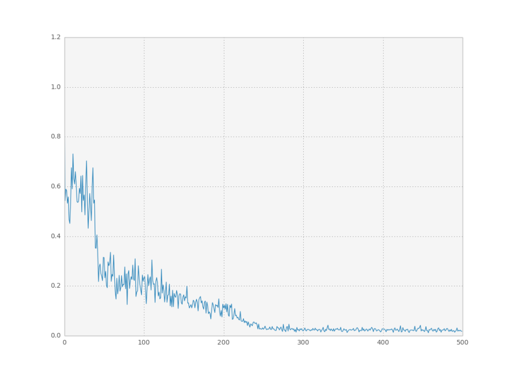
As a small test for this network I asked it to compute the dot product of two vectors, where only each dimension was provided at each time step: $\sum_{t=0}^{10} x_0^t x_1^t$. The network had to learn how to multiply the two numbers and ‘memorize’ the intermediate calculation results. This simple example works quite well:
There are many subtleties I didn’t cover here: I didn’t optimize the minibatch size in gradient descent (always set to one); and I didn’t check whether the network generalizes to different numbers of time steps after trained (probably only within a very limited range). Furthermore there’s been some really interesting research on how to avoid local minima when training recurrent nets by using simple heuristics when calculating the gradients. There is code available here which demonstrates this new method with theano: it’s really interesting, and it’s where I adapted my simple recurrent network code from. Also be sure to read this tutorial on recurrent nets for a quick overview of some basic concepts I haven’t covered here.
Additionally in a machine learning context we need to be careful with overtraining: because the training samples we have available probably do not span the whole input-output range of the system and might be corrupted with noise, the training procedure might learn to reproduce the specific data set we have but not its underlying model. There are several methods to try to counter this: separate training, test and validation datasets, or augmenting the dataset with samples corrupted with white noise.


