In systems biology we often need to solve diffusion equations of the type
where W is a white noise process; they’re the most common example of a stochastic differential equation (SDE). There are only very few cases for which we can analytically solve this equation, such as when either f or g are constant or just depend linearly on x. Of course most interesting cases involve complicated f and g functions, so we need to solve them numerically.
One way to solve this is to use a straightforward variant of the Euler method. You just need to do the usual time discretization $\delta t = T/N$ (with T the total time and N the number of steps) and then update your current value with the deterministic contribution $\delta t \times f$ and the stochastic contribution $\sqrt{\delta t} \times g$. If you are not familiar with stochastic calculus you may be wondering why is the time step multiplier $\sqrt{\delta t}$ for the stochastic part.
The equations we are interested in integrating take the general form:
a Langevin equation. $\eta$ denotes the white noise process. If we want to determine the value of x at a certain time t we just integrate the differential equation like a physicist:
with $dW=\eta(s) ds$ the integration measure. This is why sdes are commonly written in the form of the first equation of this post. Now when you express this integral as a limit of a sum of small increments of a brownian motion you can show that $dW^2 = dt$. You can find the proof in page 83 of the wonderful Gardiner.
The Euler method consists of simply replacing the integrals in the above equation with sums, obtaining the finite difference scheme
In python code this just looks like
def euler(x, dt):
	return x + dt*f(x) + sqrt(dt)*g(x)*r
With r some pseudorandom number with normal distribution. The problem with the Euler method in stochastic systems is that it fares even worse than its deterministic cousin. It strongly converges only as $O(\delta t^{\frac{1}{2}})$. The strong means that we are looking at the difference between the random variables themselves $\langle |X_t - X’_t| \rangle \leq C_t \delta t^{\frac{1}{2}}$. But because this is a stochastic system and we are simulating many paths, there is hope yet: perhaps the statistics of the values (and not the values themselves) will not be as sensitive to error. Indeed this is the case for the euler method. It has a weak convergence order of 1: $|\langle X_t \rangle - \langle X’_t \rangle| \leq C_t \delta t^1$. This means that the euler method might be appropriate if you just want the statistics of the values at a certain point, but not if you want to reconstruct the stochastic paths themselves.
As in deterministic systems, the next step up is the 4th order runge kutta. It only offers a meagre improvement though: it converges as order $O(\delta t)$ both weakly and strongly. But it’s an improvement! It is not very straightforward to implement, so I based my implementation off of Burkhardt’s code, available online.
Once we have defined the steps, we can use theano to loop through them in order and save the result. We achieve this through the use of the scan primitive:
(cout, updates) = theano.scan(fn=rk4,
			outputs_info=[c], #output shape
			non_sequences=[n, k, l, dt], #fixed parameters
			n_steps=total_steps)
There is no way to pass theano’s fast random number generator (called randomstream) directly in scan. As far as I know, you have two options: either you define it in the main code loop leaving it available as a global variable, which then allows theano to add the generator to the computational graph; or you make the stepping function part of an object, and make the randomstream a property of that object. It works out the same in practice, but the second method avoids relying on global variables, which will come back to bite you once you have a complex project with stuff scattered in different modules. For the example codes in this post I left it as global variable because they are one-off scripts.
Let’s warm up with a simple function, a bistable genetic switch:
For $n>1$, the system acts as a switch: if the concentration goes significantly above $k$ the system will be stuck at high concentrations and vice versa. I also define the system to undergo a geometric brownian walk, which just means $g \propto c$. Starting at exactly $c(0)=k$ we leave stochasticity to determine the fate of the system, which means roughly half of the trajectories will go up and half down.
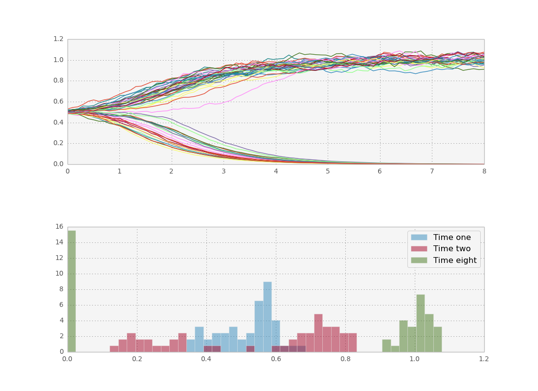
Let’s see what happens if we do more paths in parallel, to take advantage of theano.
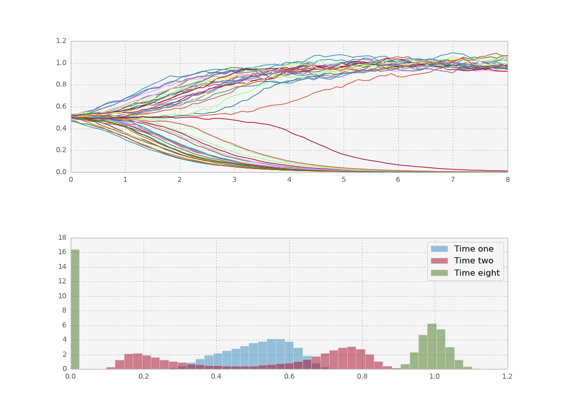
Now we reap the rewards of theano’s leveraging of fast BLAS libraries for parallel processing: even on my macbook’s cpu I can run 50.000 stochastic paths in one second. This is enough to get a smooth histogram even for later times.
We can even couple the trajectories. Let’s look at a slightly more complicated case where the function f depends on the average of the paths themselves:
Reference: A Design principle of group-level decision making in cell populations.
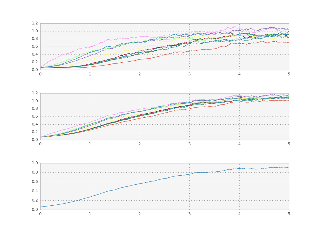
Simulation of collective decision making. First plot shows x, second s, third x average.
Below you can find the code for the bistable switch:
'''
Created on Oct 15, 2013

@author: tiago
'''
import theano
import theano.tensor as T
from theano.tensor.shared_randomstreams import RandomStreams
import numpy as np
import matplotlib.pyplot as plt
import time

#define the ode function
#dc/dt  = f(c, lambda)
#c is a vector with n components
def evolve(c, n, k, l):
	return T.pow(c, n)/(T.pow(c, n)+T.pow(k,n)) - l*c

def euler(c, n, k, l, dt):
	return T.cast(c + dt*evolve(c, n, k, l) + T.sqrt(dt)*c*rv_n, 'float32')

def rk4(c, n, k, l, dt):
	'''
	Adapted from
	http://people.sc.fsu.edu/~jburkardt/c_src/stochastic_rk/stochastic_rk.html
	'''
	a21 =   2.71644396264860
	a31 = - 6.95653259006152
	a32 =   0.78313689457981
	a41 =   0.0
	a42 =   0.48257353309214
	a43 =   0.26171080165848
	a51 =   0.47012396888046
	a52 =   0.36597075368373
	a53 =   0.08906615686702
	a54 =   0.07483912056879

	q1 =   2.12709852335625
	q2 =   2.73245878238737
	q3 =  11.22760917474960
	q4 =  13.36199560336697

	x1 = c
	k1 = dt * evolve(x1, n, k, l) + T.sqrt(dt) * c * rv_n

	x2 = x1 + a21 * k1
	k2 = dt * evolve(x2, n, k, l) + T.sqrt(dt) * c * rv_n

	x3 = x1 + a31 * k1 + a32 * k2
	k3 = dt * evolve(x3, n, k, l) + T.sqrt(dt) * c * rv_n

	x4 = x1 + a41 * k1 + a42 * k2
	k4 = dt * evolve(x4, n, k, l) + T.sqrt(dt) * c * rv_n

	return T.cast(x1 + a51 * k1 + a52 * k2 + a53 * k3 + a54 * k4, 'float32')

if __name__ == '__main__':
	#random
	srng = RandomStreams(seed=31415)

	#define symbolic variables
	dt = T.fscalar("dt")
	k = T.fscalar("k")
	l = T.fscalar("l")
	n = T.fscalar("n")
	c = T.fvector("c")

	#define numeric variables
	num_samples = 50000
	c0 = theano.shared(0.5*np.ones(num_samples, dtype='float32'))
	n0 = 6
	k0 = 0.5
	l0 = 1/(1+np.power(k0, n0))
	dt0 = 0.1
	total_time = 8
	total_steps = int(total_time/dt0)
	rv_n = srng.normal(c.shape, std=0.05) #is a shared variable

	#create loop
	#first symbolic loop with everything
	(cout, updates) = theano.scan(fn=rk4,
									outputs_info=[c], #output shape
									non_sequences=[n, k, l, dt], #fixed parameters
									n_steps=total_steps)
	#compile it
	sim = theano.function(inputs=[n, k, l, dt],
						outputs=cout,
						givens={c:c0},
						updates=updates,
						allow_input_downcast=True)

	print "running sim..."
	start = time.clock()
	cout = sim(n0, k0, l0, dt0)
	diff = (time.clock() - start)
	print "done in", diff, "s at ", diff/num_samples, "s per path"
	downsample_factor_t = 0.1/dt0 #always show 10 points per time unit
	downsample_factor_p = num_samples/50
	x = np.linspace(0, total_time, total_steps/downsample_factor_t)
	plt.subplot(211)
	plt.plot(x, cout[::downsample_factor_t, ::downsample_factor_p])
	plt.subplot(212)
	bins = np.linspace(0, 1.2, 50)
	plt.hist(cout[int(1/dt0)], bins, alpha = 0.5,
				normed=True, histtype='bar',
				label=['Time one'])
	plt.hist(cout[int(2/dt0)], bins, alpha = 0.5,
				normed=True, histtype='bar',
				label=['Time two'])
	plt.hist(cout[-1], bins, alpha = 0.5,
				normed=True, histtype='bar',
				label=['Time eight'])
	plt.legend()
	plt.show()
And for the coupled equations:
'''
Created on Jul 1, 2013

@author: tiago
'''
import theano
import theano.tensor as T
from theano.tensor.shared_randomstreams import RandomStreams
import numpy as np
import matplotlib.pyplot as plt
import time

#define the ode function
#dc/dt  = f(c, lambda)
#c is a vector with n components
def evolve(c, s, k, l):
	return T.cast((1-l)*T.pow(s, 2)/(T.pow(s, 2)+T.pow(k,2)) + l - c,'float32')

def average(c, r, g):
	n = c.shape[0]
	return T.cast(r*T.sum(c)/n + g*c,'float32')

def system(c, s, a, k, l, r, g, dt):
	return [T.cast(c + dt*evolve(c, s, k, l) + T.sqrt(dt)*c*rv_n,'float32'),
		T.cast(average(c, r, g),'float32'),
		T.cast(T.sum(c)/c.shape[0],'float32')]

if __name__ == '__main__':
	#random
	srng = RandomStreams(seed=31415)

	#define symbolic variables
	dt = T.fscalar("dt")
	k = T.fvector("k")
	l = T.fscalar("l")
	r = T.fscalar("r")
	g = T.fscalar("g")
	c = T.fvector("c")
	s = T.fvector("s")
	a = T.fscalar("a")

	#define numeric variables
	n_cells = 10
	c0 = theano.shared(np.ones(n_cells, dtype='float32')*0.05)
	s0 = theano.shared(np.ones(n_cells, dtype='float32'))
	k0 = np.random.normal(loc = 0.3, scale = 0.2, size = n_cells)
	l0 = 1/2
	r0 = 0.8
	g0 = 0.4
	dt0 = 0.01
	total_steps = 500
	rv_n = srng.normal(c.shape, std=0.1) #is a shared variable

	#create loop
	#first symbolic loop with everything
	([cout, sout, aout], updates) = theano.scan(fn=system,
											outputs_info=[c,s,a], #output shape
											non_sequences=[k,l,r,g,dt], #fixed parameters
											n_steps=total_steps)
	#compile it
	sim = theano.function(inputs=[a, k, l, r, g, dt],
						outputs=[cout, sout, aout],
						givens={c:c0, s:s0},
						updates=updates,
						allow_input_downcast=True)

	print "running sim..."
	start = time.clock()
	[cout, sout, aout] = sim(0, k0, l0, r0, g0, dt0)
	diff = (time.clock() - start)
	print "done in", diff, "s at ", diff/n_cells, "s per path"
	x = np.linspace(0, total_steps*dt0, total_steps)
	plt.subplot(311)
	plt.plot(x, cout)
	plt.subplot(312)
	plt.plot(x, sout)
	plt.subplot(313)
	plt.plot(x, aout)
	plt.show()