Suppose you are faced with a high dimensional dataset and want to find some structure in the data: often there are only a few causes, but lots of different data points are generated due to noise corruption. How can we infer these causes? Here I’m going to cover the simplest method to do this inference: we will assume the data is generated by a linear transformation of the hidden causes. In this case, it is quite simple to recover the parameters of this transformation and therefore determine the hidden (or latent) variables which represent their cause.
Mathematically, let’s say the data is given by a high-dimensional (size N) vector $u$ which is generated by a low-dimensional (size M) vector $v$ via
where $W_i$ are N-dimensional vectors which encode the transformation. For simplicity I will assume $u$ to have mean value 0. Let’s assume the noise is gaussian. Then the distribution for the data is
with $\Sigma$ a diagonal matrix. This means that we assume any correlation structure in the data arises from the transformation $W$, and not due to noise correlations. This model is the main feature of the procedure known as Factor analysis.
To fit the model we need both the weights $W$ and factors $v$ which best fit the data (in the case of no prior information for $v$, this corresponds to maximising the likelihood function). It is convenient to take the logarithm of the likelihood function:
So we are looking for $\arg\max_{W,v,\Sigma} \log P(u|v)$. The obvious way to obtain the parameters is to use expectation-maximisation: we calculate what are the factors given $W$ and $\Sigma$, and then update those parameters given the new factors in such a way as to maximise the log-likelihood. Iterating this process will result in convergence to a final set of weights and factors, which will be a local minimum of the likelihood.
Let’s examine how this works with a very simple example: the Iris dataset. This is a 4 dimensional dataset, with each dimension corresponding to a physical measurement of the sepals and petals of a flower. There are 3 different flowers so we can assume that each flower’s genome will code for different physical features. So the question is whether there is a ‘genome variable’ $v$ which maps into the observed physical features $u$? Let’s load the dataset directly using sklearn:
from sklearn import datasets

iris = datasets.load_iris()
x = iris.data # physical measurements
y = iris.target # actual species for visualization
And now we can plug this directly into the Factor analysis model:
import matplotlib.pyplot as plt
from sklearn.decomposition import FactorAnalysis

model = FactorAnalysis(n_components=2)
x_reduced = model.fit_transform(x)
plt.scatter(x_reduced[:, 0], x_reduced[:, 1], c=y, cmap=plt.cm.Paired)
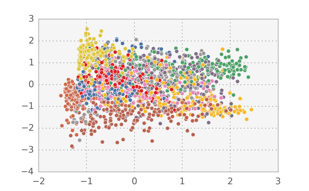
Let’s visualize the hidden factors for the actual data points we have by inverting the transformation. Below you can see the data with $v_1$ in the x-axis and $v_2$ in the y-axis.
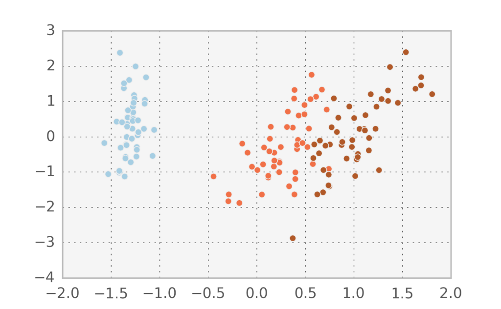
In fact, it seems that the first component $v_1$ manages to describe accurately the variation between the 3 different species. Let’s try to do Factor analysis with just one component and see what comes out (I added some randomness in the y-direction to visualize the points better).
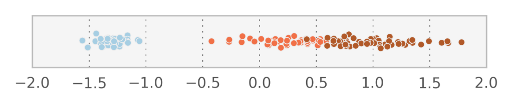
With 1 component we obtain an estimate for $\Sigma^{-1} = [ 0.16350346, 0.15436415, 0.00938691, 0.04101233]$ which corresponds to the variation of the data which is not explained by the linear transformation of $v$. What if we would force all diagonal elements of $\Sigma$ to be identical? In that case, we observe that the vectors $W_i$ actually form an orthogonal basis (i.e. each one is perpendicular to the next). This in turn means that when we project the data to the space of the hidden variables, each $v_i$ will be uncorrelated to the others (which does not happen with Factor analysis).
Linear algebra explains why this happens: after some calculation, we can observe that the obtained $W_i$ correspond to the principal eigenvectors (i.e. are associated to the largest eigenvalues) of the sample covariance matrix $C= \frac{1}{N}\sum_{j=1}^N (u^j - \bar{u}) (u^j-\bar{u})^T$ with the overscripts denoting sample index. This method has a specific name and is called Probabilistic Principal Components Analysis. Setting $\Sigma = 0$ we obtain the popular vanilla PCA.
Typically we sort the eigenvectors such that $W_1$ corresponds to the largest eigenvalue of $C$ meaning that the hidden variable $v_1$ explains the most variation in the observed data. Now $W_2$ must be perpendicular to $W_1$, which means that $v_2$ will explain the most remaining variation in the data, and so on. If we allow $M=N$ then it would be possible to completely reconstruct the data from $v$.
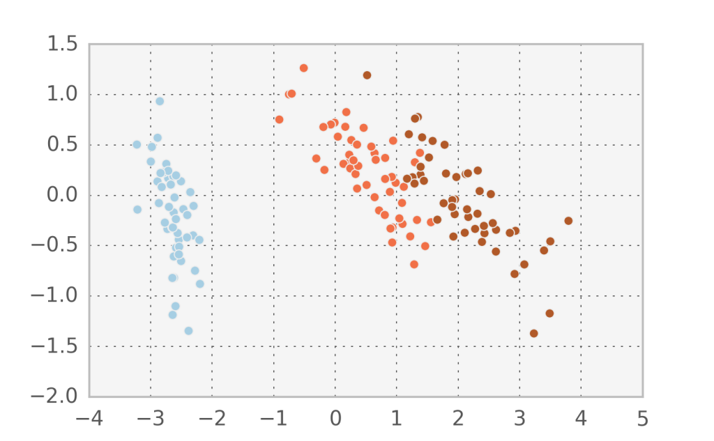
In the Iris dataset we can observe that the projected subspace using probabilistic PCA is different to the one found in Factor analysis. We can confirm that we found orthogonal components by printing $W_1 \cdot W_2$ and comparing it to Factor analysis:
model = PCA(n_components=2)
x_reduced = model.fit_transform(x)
print np.dot(model.components_[0], model.components_[1])
# 3.43475248243e-16

model = FactorAnalysis(n_components=2)
x_reduced = model.fit_transform(x)
print np.dot(model.components_[0], model.components_[1])
# 0.146832660483
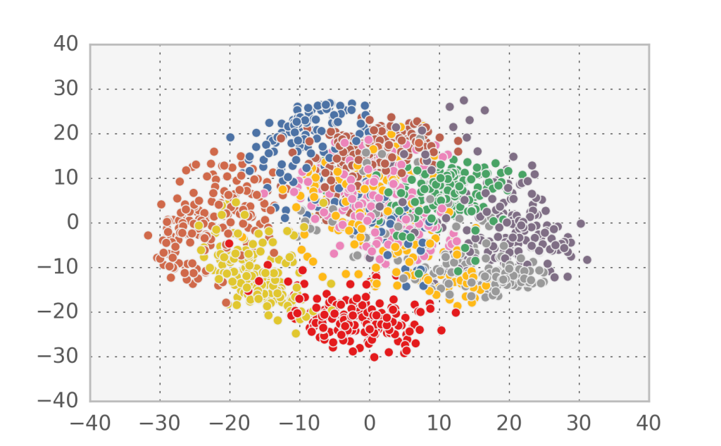
In the case of handwritten digits, the first two components in PCA appear to capture more of the structure of the problem than the first two factors in factor analysis. However, since this is a strongly nonlinear problem, none of them can accurately separate all 10 digit classes.
If we look at the log-likelihood equivalent for PCA we observe a very deep connection: $\log P(u|v) = -\frac{1}{2}(u-W\cdot v)^2$. The $W, v$ that come out of PCA (i.e. maximise the log-likelihood) also minimize the least squares reconstruction error for the simplest linear model. From a data compression perspective, that means that we can compress the information contained in $u$ by saving only $W$ and $v$. This is worth it when we have a large number of samples of $u$, since $W$ is constant and each $v$ is smaller than each $u$.
With the fit distribution in hand, we can even generate new samples of $u$. We just need to draw some samples of low-dimensional $v$ and pass it through the linear model we have. Let’s see what happens when we apply this idea to the digits dataset, sampling $v$ from a gaussian approximation of the $v$ corresponding to the actual data distribution.
v = model.transform(x)
v_samples = np.random.multivariate_normal(
    np.mean(v, axis=0), np.cov(v.T), size=100)
x_samples = model.inverse_transform(v_samples)
To finish this long post, let’s just look at what happens if we don’t assume a flat prior for $v$. Two common options are to assume $P(v)$ is a gaussian or an exponential distribution. Then the log-likelihood (getting rid of constants, as usual) becomes:
Those two terms correspond to the often used $L_2$ and $L_1$ regularization, which for linear models have the fancy names of ridge regression and lasso respectively (not really sure why they need fancy names). Writing this in a more CS notation, we can say that our problem consists of maximising:
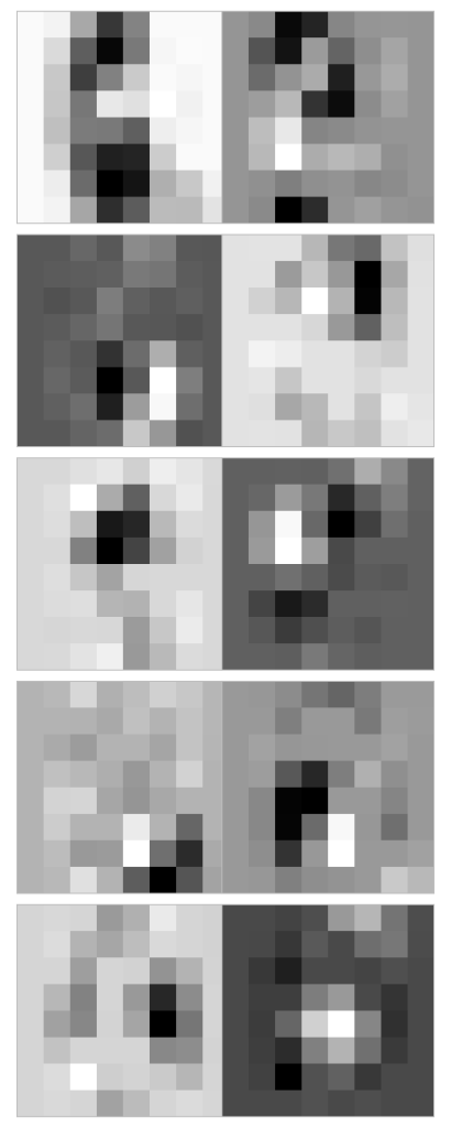
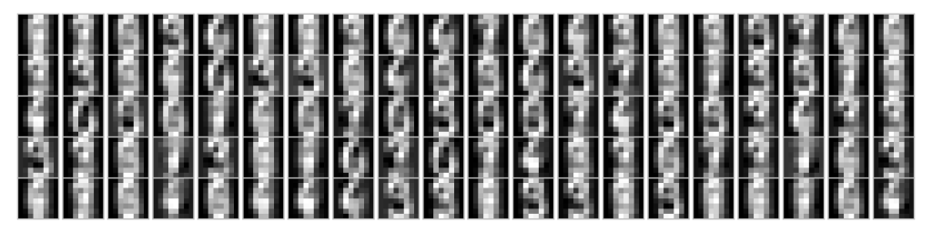
This problem has been given the name of Sparse PCA, and we can find an implementation in scikits. Let’s see what happens when we apply it to the digits dataset.
from sklearn.decomposition import SparsePCA
from sklearn import datasets

dset = datasets.load_digits()
x = dset.data
y = dset.target

model = SparsePCA(n_components=10, alpha=0)
x_reduced = model.fit_transform(x)

print np.dot(model.components_[0], model.components_[1])

n_row = 5
n_col = 2
plt.figure(figsize=(6, 15))
for i in xrange(10):
	comp = model.components_[i]
	plt.subplot(n_row, n_col, i + 1)
	vmax = max(comp.max(), -comp.min())
	plt.imshow(comp.reshape([8,8]), cmap=plt.cm.gray, interpolation='nearest')
	plt.xticks(())
	plt.yticks(())
plt.tight_layout()
plt.savefig('digits_SPCA_rec.png')
Immediately we notice that we lose the orthogonality of the components due to the constraints. Let’s see how they look like: