Wiener filter
The wiener filter is a bit more advanced than the filters I previously covered, as it is the first one rooted in probability theory. Consider a more complicated measurement, $y = r*s + n$, where $R$ is an operator describing the response of the measurement equipment (for images, it is known as point spread function). We want to find the signal estimate $\hat{s}$ which minimizes the distance
i.e., the minimum mean square error. This estimate should be given for a linear filter $w$ such that $\hat{s} = w*y$.
Since we are working with convolutions is convenient to work in frequency space. Thus our equations will be (I’ll use the all caps convention to denote the fourier transform, as it appears to be the norm in signal processing literature): $\hat{S} = W Y$. It is also helpful to know about the
Wiener-Khinchin theorem, which relates the power spectrum of a stochastic process with the fourier transform of its autocorrelation: $P_{yy}=Y^*Y=|Y|^2$, where the asterisk denotes complex conjugate. Note we could also use this to calculate cross correlations, hence the subscript with two letters. So, in fourier space, the wiener filter $W$ will be given by:
A derivation is given in wikipedia. If there was no noise ($P_{nn}=0$), the filter would just be a deconvolution of the original transformation: $W=1/R$. When there is noise, the filter essentially only passes through frequencies for which the signal to noise ratio is high ($\frac{P_{nn}}{P_{ss}}\simeq 0$), while attenuating others proportionally to the noise power. Often we don’t know the power spectrum of the original signal so we must provide some sort of estimate. If the noise process is white, then $P_{nn}=\sigma^2$ and we simplify the filter by assuming the signal also has a constant power spectrum (i.e. we are totally ignorant about which frequencies are more powerful or not). Thus the filter becomes simply
where $K$ is provided by the user. SciPy takes this simplification to the extreme, and their implemented filter is:
with $\sigma^2$ provided by the user and $m_x$ and $\sigma_{x}^{2}$ are locally estimated with $N$ data points, also provided by the user. Let’s see how this works out:
def testWiener(x, y, s, npts):
	wi = wiener(y, mysize=29, noise=0.5)
	plt.plot(x,wi)
	print "wieerr", ssqe(wi, s, npts)
	return wi
I passed the correct variance for the simulated noise process. If you leave this parameter blank, the wiener filter is just a gaussian average. You need to play with the window around a bit, as with the previous filters we discussed. But in the end we get the same performance as before.
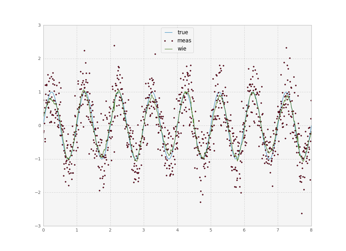
I was quite disappointed with the performance of this filter, since it requires the same amount of information input as the classic filters with no accuracy gain. I suspect this is due to scipy’s shady implementation though, and a more rigorous frequency space implementation might work a bit better.
Splines
A final smoothing method I want to discuss is the use of smoothing splines. This method is more of a heuristic when compared to others, since splines are not directly related to any kind of frequency analysis or probability theory. However, by clever use of optimization methods we can effectively use them to obtain an approximation to a signal.
First a quick intro to splines. The most commonly used splines are Bézier splines and B splines, a generalization of the first. Bézier splines are constructed by creating a series of Bézier curves such that they join at their endpoints, usually in such a way that the curve is $C^1$ continuous. Such a Bézier curve with $N$ control points in the range $[0,1]$ is equal to a Bspline with degree $N-1$. Here is a comparison between a bézier curve and a Bspline:
Bez[x_, p_] :=
  Sum[BernsteinBasis[Length[p] - 1, i - 1, x]*p[[i]], {i,
    Length[p]}];
source = {1, 8, 4, 2, 5, 8, 4};
sparam = Table[{(i - 1)/(Length[source] - 1), source[[i]]}, {i,
    Length[source]}];
f = BSplineFunction[source,
   SplineDegree -> 1];(*same as linear interp*)

b = BSplineFunction[source,
   SplineDegree -> (Length[source] - 1)];(*same as bezier*)
Show[
 Graphics[{Red, Point[sparam], Green, Line[sparam]}, Axes -> True,
  AspectRatio -> 1/1.6],
 Plot[{f[x], b[x], Bez[x, source]}, {x, 0, 1}], AspectRatio -> 1/1.6]
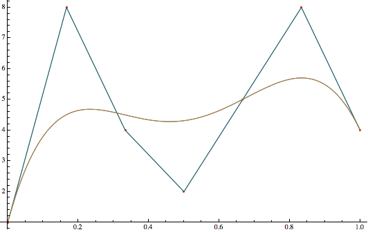
When we need smooth and complex curves, it is preferable to use a single Bspline instead of joining many Bézier curves together since less parameters are necessary. If we have N control points and a degree k, then the bézier curve needs $k+1$ parameters for each segment. Ignoring repeats, that’s a total of $(N-1)k+1$ while the Bspline needs only $N+k-1$ parameters. Since we are talking about a curve in the (x,y) plane, each parameter is of course a vector of two real numbers.
To solve our smoothing problem, we pick a number N of control points (which defines how smooth the curve is) and fix a degree (as low as possible, often 3) and let an optimization routine pick the right parameters such that E[(s(y)-y)^2] is minimized. The big advantage of this method is that we get a result with a very low number of parameters compared to the others (which have essentially as many parameters as number of data points) and we get a smooth function which we can integrate, derive or whatever we want. Here is a function I wrote which receives a number of points from an optimization algorithm and constructs a valid spline approximation (in this particular case I constrained the first and last points and sorted the x points, hence the complication in the code) in GSL.
In python, our life is made much easier by a built in function, UnivariateSpline. This function performs the algorithm I described just above, with the difference that you can’t directly pick the number of control points. Rather it asks for a parameter which picks the correct number of control points to satisfy a smoothing condition. While this is useful for novice users, I wish there would be an option to either directly set the number of control points, or normalize the smoothing condition by the number of points. The way the function works now means that if I increase the number of points sampled in a fixed interval I need to reset s for a given target smoothness. Also, since s depends on the sum of squared errors, different datasets will give different results. Alas, let’s try it:
def testSpline(x, y, s, npts):
	sp = UnivariateSpline(x, y, s=240)
	plt.plot(x,sp(x))
	print "splerr", ssqe(sp(x), s, npts)
	return sp(x)

While the end result looks much better than the previous methods, the error is actually roughly the same as for all other options we tried out. I have not yet discussed wavelet analysis, but it is a framework more often applied to image processing than to time series so I will leave it for a future, unrelated post. Thus it seems we hit a brick wall with respect to model free methods. It looks like the best way forward to improve accuracy is to introduce more information into the method by providing a mathematical model of the system in study. Indeed, these methods have become more and more popular in the past years due to the surge in computing power. I’ll discuss these methods in a next post. For reference, here is the full python code used to produce the plots I’ve been showing.
'''
Created on Mar 16, 2013

@author: tiago
'''

import numpy as np
from scipy.interpolate import UnivariateSpline
from scipy.signal import wiener, filtfilt, butter, gaussian, freqz
from scipy.ndimage import filters
import scipy.optimize as op
import matplotlib.pyplot as plt

def ssqe(sm, s, npts):
	return np.sqrt(np.sum(np.power(s-sm,2)))/npts

def testGauss(x, y, s, npts):
	b = gaussian(39, 10)
	#ga = filtfilt(b/b.sum(), [1.0], y)
	ga = filters.convolve1d(y, b/b.sum())
	plt.plot(x, ga)
	print "gaerr", ssqe(ga, s, npts)
	return ga

def testButterworth(nyf, x, y, s, npts):
	b, a = butter(4, 1.5/nyf)
	fl = filtfilt(b, a, y)
	plt.plot(x,fl)
	print "flerr", ssqe(fl, s, npts)
	return fl

def testWiener(x, y, s, npts):
	wi = wiener(y, mysize=29, noise=0.5)
	plt.plot(x,wi)
	print "wieerr", ssqe(wi, s, npts)
	return wi

def testSpline(x, y, s, npts):
	sp = UnivariateSpline(x, y, s=240)
	plt.plot(x,sp(x))
	print "splerr", ssqe(sp(x), s, npts)
	return sp(x)

def plotPowerSpectrum(y, w):
	ft = np.fft.rfft(y)
	ps = np.real(ft*np.conj(ft))*np.square(dt)
	plt.plot(w, ps)

if __name__ == '__main__':
	npts = 1024
	end = 8
	dt = end/float(npts)
	nyf = 0.5/dt
	sigma = 0.5
	x = np.linspace(0,end,npts)
	r = np.random.normal(scale = sigma, size=(npts))
	s = np.sin(2*np.pi*x)#+np.sin(4*2*np.pi*x)
	y = s + r
	plt.plot(x,s)
	plt.plot(x,y,ls='none',marker='.')
	ga = testGauss(x, y, s, npts)
	fl = testButterworth(nyf, x, y, s, npts)
	wi = testWiener(x, y, s, npts)
	sp = testSpline(x, y, s, npts)
	plt.legend(['true','meas','gauss','iir','wie','spl'], loc='upper center')
	plt.savefig("signalvsnoise.png")
	plt.clf()
	w = np.fft.fftfreq(npts, d=dt)
	w = np.abs(w[:npts/2+1]) #only freqs for real fft
	plotPowerSpectrum(s, w)
	plotPowerSpectrum(y, w)
	plotPowerSpectrum(ga, w)
	plotPowerSpectrum(fl, w)
	plotPowerSpectrum(wi, w)
	plotPowerSpectrum(sp, w)
	plt.yscale('log')
	plt.xlim([0,10])
	plt.ylim([1E-8,None])
	plt.legend(['true','meas','gauss','iir','wie','spl'], loc='upper center')
	plt.savefig("spectra.png")