Last time we started talking about state space models with the Kalman Filter. Our aim has been to find a smoothed trajectory for some given noisy observed data. In the case of state space models, we incorporate a model for the underlying physical system to calculate a likelihood for each trajectory and select the optimal one. When it comes to implementing this idea, we run into the problem of how to represent the probability distributions for the state of the system: it would be unfeasible to calculate the probability for every single point in phase space at all times. The Kalman filter solves this by approximating the target probability density function (abbreviated pdf) with a Gaussian, which has only two parameters. This approximation works surprisingly well but it might not be optimal for cases where the underlying pdf is multimodal.
Today we will be looking at another idea to implement state space models - the particle filter. Our goal is still to find the maximum of the posterior distribution $P(x|y,\theta)$, given by bayes’ formula:
Now the idea is to approximate this distribution by randomly drawing points from it. Because we will only look at one time step at a time, the sequence of points we sample will be a markov chain; and because the method relies on random sampling we call it a markov chain monte carlo (MCMC) method.
Formally, consider the expectation of a function f at some time point:
We can approximate this integral by sampling a bunch of points according to $p(x|y)$ and then approximating the integral with the sum $\sum_{j}f(x^j)$. Note that when f is a delta function we are sampling the pdf itself. If we sample infinite points, the result will be exact; we hope we can get away with a smaller number than that. The problem is that often we don’t know how to sample from p, so we have to be clever.
The standard way to be clever is by using importance sampling. Instead of sampling directly from $p$ we sample from an easier distribution to work with: $q$, the proposal. We put it in by using a great trick: multiplying by one ($1=\frac{q}{q}$)
where w is the ratio between p and q. If we pick a nice q, the sampled points will be highly informative and we won’t need to sample quite so many points to describe the posterior distribution well. Designing a nice proposal distribution is almost an art form (or black magic?).
Let’s do this one step at a time: for each time slice, we want to sample from $P(x_i|y_{0:i})$. All we know is the distribution in the past and the new data $y_i$. Because this is a markov chain, the current value only depends on the previous value; and we know how to move from the one time point into the future: we use the chapman-kolmogorov relation
At this point it will be helpful to again multiply stuff by one. The first pdf will be the target of our sampling so we multiply and divide by $q(x_i|x_{i-1}, y_{0:i})$. We handle the second pdf by multiplying and dividing by something we should know, $P(x_{i-1}|y_{0:i-1})$. So the whole thing now looks like
Almost there! Now we use the fact that we are representing both the current time and the previous time with particles. We can use a delta function to represent the function itself with the particle set
And recognize that the integral over $x_{i-1}$ is an expectation over the pdf of the previous time, which is also represented by particles. It then becomes
That’s a lot of particles! Now there is an obvious simplification: because in the computer we only evolve one particle at a time, there will be only one $x^j_{i-1}$ that resulted in a given $x^n_{i}$. Thus the inner sum is approximated as being over only one particle which makes the sum go away.
So we can sample according to $q(x_i|x_{i-1}, y_{0:i})$ and the weights will be given by what remains. We can rewrite the weights as
</span>(we can ignore the normalization because we can renormalize them at the end). We still need to use black magic to determine the sampling distribution $q(x_i|x_{i-1}, y_{0:i})$, but often we cheat and use $P(x_{i-1}|y_{0:i-i})$, which makes the weights $w\propto w(x^n_{i-1})P(y_i|x_i)$.
One problem is that samples tend to accumulate in regions in phase space with large probability. It might happen that after some time steps we have only one particle with weight approximately 1 and all others 0. To fix this we can, at each time step, resample the particle set according to the current probability distribution, which then resets all the weights: $w(x^n) = 1/N$. Hopefully these particles will be better at exploring the phase space.
Let’s try this algorithm on the nonlinear problem which stumped the Kalman filter. As before, we use as transition function $p(x_i|x_{i-1})$ the integral of the differential equations for the van der pol oscillator. You can find the python code on github.
The result is more a testament to how amazing an approximation the Kalman Filter is than anything else: the particle filter manages an mse of 0.108 vs. the Kalman filter’s 0.123 when the nonlinearity parameter is set to 4. I guess my experiments are probably too easy for these advanced methods. You can visualize the particles evolving along time in the following plot:
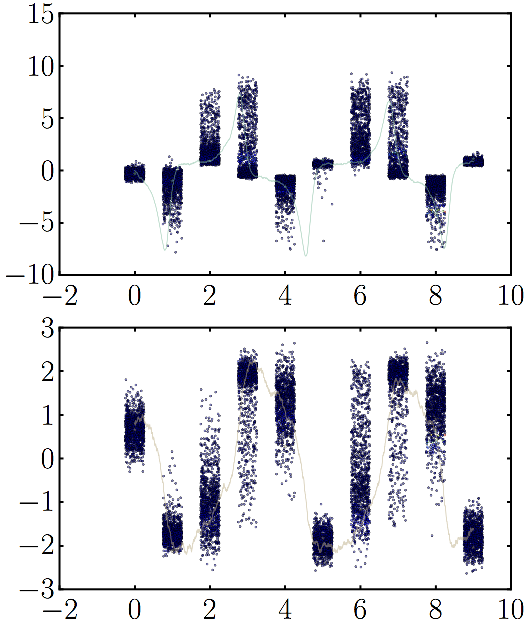
Visualization of particle set evolution for a single nonlinear van der pol oscillator. I dispersed the points for each time step a little around t to make the distribution easy to see, but there are only 10 measurements total (corresponding to each of the clusters). Notice the nice quenching in position space due to the dynamics all converging to that point in phase space. The particles are also colored by weight but you can barely see the points with significantly higher weights among all the samples. 1000 particles total.
A caveat for these methods is that we must know the underlying parameters for the physical system if they are to work well. In many situations, there is a way to estimate them, but in others we actually need the smoothed result to estimate the parameters, such as in systems biology. In a future post I will talk about the challenges of parameter inference for state space models.