Sometimes you need to estimate a probability distribution from a set of discrete points. You could build a histogram of the measurements, but that provides little information about the regions in phase space with no measurements (it is very likely you won’t have enough points to span the whole phase space). So the data set must be smoothed, as we did with time series. As in that case, we can describe the smoothing by a convolution with a kernel. In this case, the formula is very simple \(f(x)=\frac{1}{N}\sum_i^N K(x-x_i)\)
The choice of K is an art, but the standard choice is the gaussian kernel as we’ve seen before. Let’s try this out on some simulated data
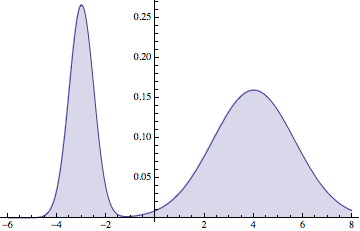
d = MixtureDistribution[{1, 2}, {NormalDistribution[-3, 1/2],
    NormalDistribution[4, 5/3]}];
Plot[Evaluate[PDF[d, x]], {x, -6, 8}, Filling -> Axis]
And now let’s apply KDE to some sampled data.
ns = 100;
dat = RandomVariate[d, ns];
\[Sigma] = 1;
c[x_] := Sum[
Exp[-(dat[[i]] - x)^2/(2*\[Sigma])]/(Sqrt[2 \[Pi] \[Sigma]]), {i,
ns}];
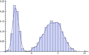
Show[Histogram[dat, 30, "ProbabilityDensity"],
Plot[c[x]/ns, {x, -6, 8}]]
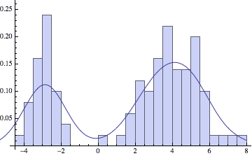
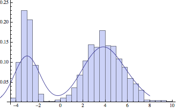
The choice of standard deviation makes a big difference in the final result. For low amounts of data we want a reasonably high sigma, to smoothen out the large variations in the data. But if we have a lot of points, a lower sigma will more faithfully represent the original distribution: