In the previous post, I showed how to efficiently solve SDEs using python. Today we will use that knowledge to explore a well known model in systems biology: the repressilator.
The repressilator was described in detail by Elowitz and Leibler in Nature. It is essentially a simple way for a cell to create an oscillator by changing the concentration of a number of proteins by the mechanism of gene expression. It has proven to be a difficult model to recreate in practice using synthetic biology, so nobody knows if it is an accurate model of what actually happens inside the cells. But it’s simple to model using differential equations and we’re physicists (yes, you too! for now at least) so let’s have a go at it! The system is composed of N proteins, each of which is repressed by another in the set cyclically. Following the usual hill equation model for gene expression and taking into account that proteins degrade after some time, we can write the sde for the system as such:
\( c_i = \frac{k^n}{c_j^n+k^n} - c_i \lambda + c_i \eta_i\) with $j=i+1 \mod N$
The only conceptual change in the code is that now we are solving a multidimensional SDE, whereas previously we had only one variable of interest to integrate. Which means that to integrate many paths simultaneously the dynamic variable becomes a matrix instead of a vector. And that’s it! The rest of the code stays exactly the same. To define the function f I needed to use a small trick to be able to couple the variables. The problem stems from the fact that you cannot directly access matrix elements in theano so you can’t write something like c[0, t] = c[0, t-1] + dt * f(c[0, t]). Because each variable depends only on the previous one however, we can circumvent this limitation by first computing f for all elements and then rotating the whole matrix around by one, so that everyone is in the proper place. Here’s that code:
def evolve(c, n, k, l):
	hill = T.pow(k,n)/(T.pow(c, n)+T.pow(k,n))
	rep = T.roll(hill, 1, axis=1)
	return rep - l*c
Here is a sample solution:
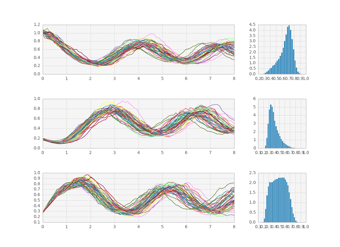
We can also plot histograms for all times, save them as individual frames, and then create an animation with imagemagick.
Full code below:
'''
Created on Oct 16, 2013

@author: tiago
'''
import theano
import theano.tensor as T
from theano.tensor.shared_randomstreams import RandomStreams
import numpy as np
import matplotlib.pyplot as plt
import matplotlib.gridspec as gridspec
import time

#define the ode function
#dc/dt  = f(c, lambda)
#c is a vector with n components
def evolve(c, n, k, l):
	hill = T.pow(k,n)/(T.pow(c, n)+T.pow(k,n))
	rep = T.roll(hill, 1, axis=1)
	return rep - l*c

def euler(c, n, k, l, dt):
	return T.cast(c + dt*evolve(c, n, k, l) + T.sqrt(dt)*c*rv_n, 'float32')

def rk4(c, n, k, l, dt):
	'''
	Adapted from
	http://people.sc.fsu.edu/~jburkardt/c_src/stochastic_rk/stochastic_rk.html
	'''
	a21 =   2.71644396264860
	a31 = - 6.95653259006152
	a32 =   0.78313689457981
	a41 =   0.0
	a42 =   0.48257353309214
	a43 =   0.26171080165848
	a51 =   0.47012396888046
	a52 =   0.36597075368373
	a53 =   0.08906615686702
	a54 =   0.07483912056879

	q1 =   2.12709852335625
	q2 =   2.73245878238737
	q3 =  11.22760917474960
	q4 =  13.36199560336697

	x1 = c
	k1 = dt * evolve(x1, n, k, l) + T.sqrt(dt) * c * rv_n

	x2 = x1 + a21 * k1
	k2 = dt * evolve(x2, n, k, l) + T.sqrt(dt) * c * rv_n

	x3 = x1 + a31 * k1 + a32 * k2
	k3 = dt * evolve(x3, n, k, l) + T.sqrt(dt) * c * rv_n

	x4 = x1 + a41 * k1 + a42 * k2
	k4 = dt * evolve(x4, n, k, l) + T.sqrt(dt) * c * rv_n

	return T.cast(x1 + a51 * k1 + a52 * k2 + a53 * k3 + a54 * k4, 'float32')

if __name__ == '__main__':
	#random
	srng = RandomStreams(seed=31415)

	#define symbolic variables
	dt = T.fscalar("dt")
	k = T.fscalar("k")
	l = T.fscalar("l")
	n = T.fscalar("n")
	c = T.fmatrix("c")

	#define numeric variables
	num_samples = 50000
	init = np.ones((num_samples, 3), dtype='float32')
	init[:, 1:3] = 0.2
	c0 = theano.shared(init)
	n0 = 6
	k0 = 0.5
	l0 = 1/(1+np.power(k0, n0))
	dt0 = 0.1
	total_time = 8
	total_steps = int(total_time/dt0)
	rv_n = srng.normal(c.shape, std=0.1) #is a shared variable

	#create loop
	#first symbolic loop with everything
	(cout, updates) = theano.scan(fn=rk4,
									outputs_info=[c], #output shape
									non_sequences=[n, k, l, dt], #fixed parameters
									n_steps=total_steps)
	#compile it
	sim = theano.function(inputs=[n, k, l, dt],
						outputs=cout,
						givens={c:c0},
						updates=updates,
						allow_input_downcast=True)

	print "running sim..."
	start = time.clock()
	cout = sim(n0, k0, l0, dt0)
	diff = (time.clock() - start)
	print "done in", diff, "s at ", diff/num_samples, "s per path"

	downsample_factor_t = 0.1/dt0 #always show 10 points per time unit
	downsample_factor_p = num_samples/50

	x = np.linspace(0, total_time, total_steps/downsample_factor_t)
	gs = gridspec.GridSpec(3, 2, width_ratios=[4,1])

	plt.subplot(gs[0, 0])
	plt.plot(x, cout[::downsample_factor_t, ::downsample_factor_p, 0])
	plt.subplot(gs[1, 0])
	plt.plot(x, cout[::downsample_factor_t, ::downsample_factor_p, 1])
	plt.subplot(gs[2, 0])
	plt.plot(x, cout[::downsample_factor_t, ::downsample_factor_p, 2])

	plt.subplot(gs[0, 1])
	plt.hist(cout[-1,:,0], 30,
				normed=True, histtype='bar')
	plt.subplot(gs[1, 1])
	plt.hist(cout[-1,:,1], 30,
				normed=True, histtype='bar')
	plt.subplot(gs[2, 1])
	plt.hist(cout[-1,:,2], 30,
				normed=True, histtype='bar')

	#plt.show()
	plt.clf()
	bins = np.linspace(0.1 , 1, 50)
	for i in xrange(cout.shape[0]):
		plt.hist(cout[i,:,1], bins,
				normed=True, histtype='bar')
		plt.xlim([0.1, 1])
		plt.ylim([0, 10])
		plt.savefig("pics/rep"+str(i)+".png")
		plt.clf()