I already talked about MCMC methods before, but today I want to cover one of the most well known methods of all, Metropolis-Hastings. The goal is to obtain samples according to to the equilibrium distribution of a given physical system, the Boltzmann distribution. Incidentally, we can also rewrite arbitrary probability distributions in this form, which is what allows for the cross pollination of methods between probabilistic inference and statistical mechanics (look at my older post on this). Since we don’t know how to sample directly from the boltzmann distribution in general, we need to use some sampling method.
The easiest would be to do rejection sampling. Draw a random number x uniformly and reject it with probability P(x). For high dimensional systems, this would require an astronomical number of samples, so we need to make sure we draw samples likely to get accepted. To do so, we draw the samples from a markov chain: a stochastic process which moves from one state of the system (i.e. a given configuration of variables) to another arbitrary state with some probability. Intuitively, if we set up the markov chain so that it moves preferentially to states close to the one we were in, they are more likely to get accepted. On the other hand, the samples will be correlated, which means we cannot draw all samples generated by the chain, but need to wait some time after drawing a new independent sample (given by the autocorrelation of the chain).
The markov chain needs to obey certain principles: ergodicity, which means the chain is able to reach all states in the system from any initial state (to guarantee the probability distribution is represented correctly); and detailed balance, which means the probability of going from state A to state B is the same as that of from state B to A, for all pairs of states in the system. This makes sure the chain doesn’t get stuck in a loop where it goes from A to B to C and back to A. Mathematically, the probabilities must obey
for the boltzmann distribution.
Now, any markov chain with those properties will converge to the required distribution, but we still haven’t decided on a concrete transition rule $p_{A\rightarrow B}$. The clever part about metropolis hastings comes now. Once a new state B has been proposed, we can actually choose to not transition to it, and instead stay where we are without violating detailed balance. To do so, we define the acceptance ratio A and the proposal distribution g. The two of them must be balanced such that
We can choose a symmetric g for simplicity, such that $g_{A\rightarrow B}=g_{B\rightarrow A}$, and thus g cancels out. Then
Now what we want is to accept as many moves as possible, so we can set one of the A’s to 1 and the other to the value on the right hand side of the equation. Because the most likely states of the system are the ones with low energy, we generally want to move in that direction. Thus we choose the A’s to follow the rule
Again, this rule actually applies to any probability distribution, since you can go back and forth from the boltzmann form to an arbitrary distribution. Let’s look at how to implement this for a simple gaussian mixture. (The code is not very well optimized, but it follows the text exactly, for ease of understanding)
import numpy as np
import matplotlib.pyplot as plt
import matplotlib.mlab as mlab

def q(x, y):
    g1 = mlab.bivariate_normal(x, y, 1.0, 1.0, -1, -1, -0.8)
    g2 = mlab.bivariate_normal(x, y, 1.5, 0.8, 1, 2, 0.6)
    return 0.6*g1+28.4*g2/(0.6+28.4)

'''Metropolis Hastings'''
N = 100000
s = 10
r = np.zeros(2)
p = q(r[0], r[1])
print p
samples = []
for i in xrange(N):
    rn = r + np.random.normal(size=2)
    pn = q(rn[0], rn[1])
    if pn >= p:
        p = pn
        r = rn
    else:
        u = np.random.rand()
        if u < pn/p:
            p = pn
            r = rn
    if i % s == 0:
        samples.append(r)

samples = np.array(samples)
plt.scatter(samples[:, 0], samples[:, 1], alpha=0.5, s=1)

'''Plot target'''
dx = 0.01
x = np.arange(np.min(samples), np.max(samples), dx)
y = np.arange(np.min(samples), np.max(samples), dx)
X, Y = np.meshgrid(x, y)
Z = q(X, Y)
CS = plt.contour(X, Y, Z, 10)
plt.clabel(CS, inline=1, fontsize=10)
plt.show()
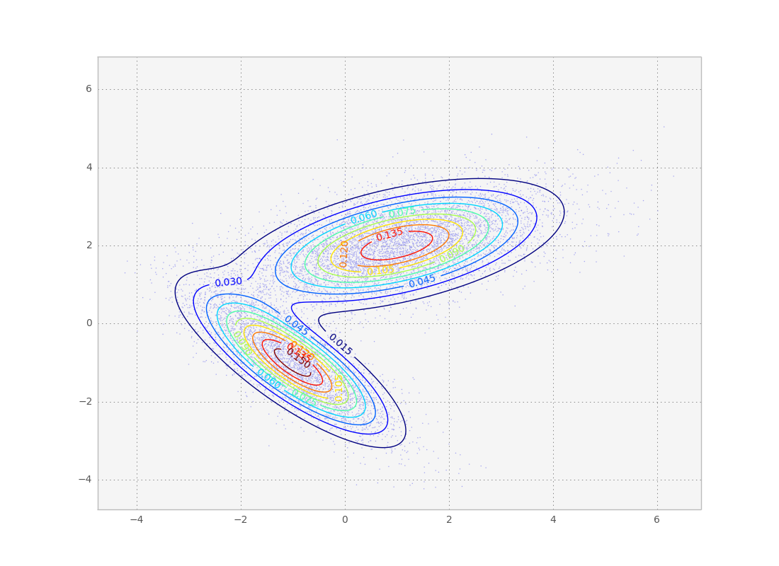
Result of the above code. As we wanted, the individual samples follow the desired probability distribution.
I guesstimated a reasonable value for the sampling rate (1 sample every 10 steps), but you could more rigorously calculate the autocorrelation for the markov chain and fit it to an exponential to get a correlation time estimate which is be a more appropriate guess. To do that, you need to calculate the autocorrelation of some observable of the probability distribution (i.e. the energy E). In this gaussian case, the autocorrelation time is so small I couldn’t even fit an exponential to the autocorrelation time the observables I tried.