Usually we like to model probability distributions with gaussian distributions. Not only are they the maximum entropy distributions if we only know the mean and variance of a dataset, the central limit theorem guarantees that random variables which are the result of summing many different random variables will be gaussian distributed too. But what to do when we have multimodal distributions like this one?
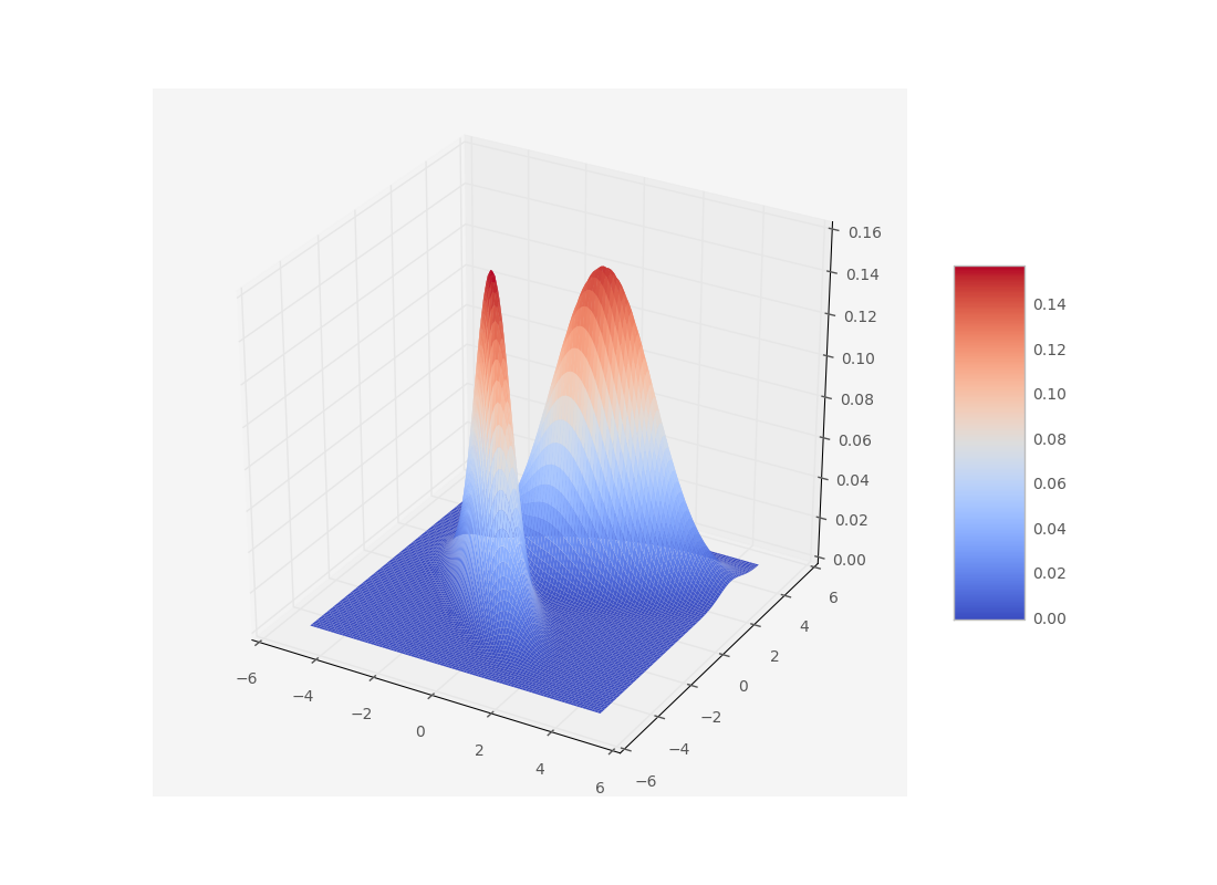
A gaussian distribution would not represent this very well. So what’s the next best thing? Add another gaussian! A gaussian mixture model is defined by a sum of gaussians
with means $\mu$ and covariance matrices $\Sigma$.
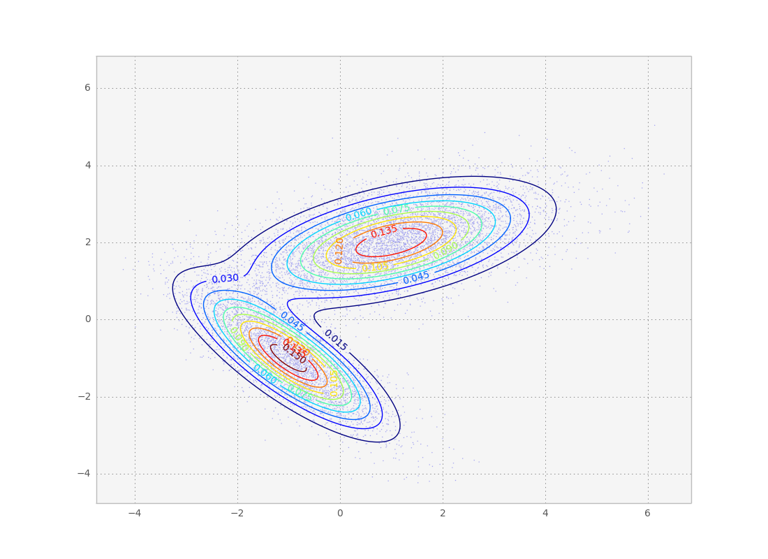
The above gaussian mixture can be represented as a contour plot. Note this is the same distribution we sampled from in the metropolis tutorial.
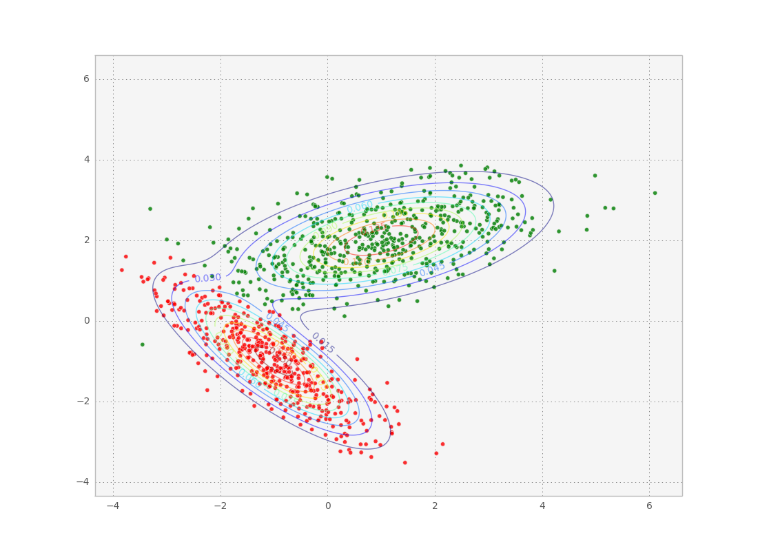
By fitting a bunch of data points to a gaussian mixture model we can then access the means and covariances of the individual modes of the probability distribution. These modes are a good way of clustering the data points into similar groups. After the fit, we can even check out to which mode each data point belongs the best by calculating the maximum of its class probability:
So how do we obtain a gaussian mixture fit to a set of data points? The simplest way is to use the maximum a priori estimate to find the set of parameters which best describe the points, i.e.
If we don’t have a prior (i.e. it is constant), this is just the maximum likelihood estimate:
There is a straightforward iterative method to obtain these estimates, the expectation-maximization algorithm. It consists of an expectation step, which calculates the likelihood for the current parameter set averaged over any latent variables in the model; and a maximization step which maximizes the parameters w.r.t. that likelihood. In this case, we consider the mode assignment $i$ to be a discrete latent variable. So intuitively, first we calculate how strongly to which mode each data point ‘belongs’, sometimes called the responsibility (expectation step). Knowing that, we calculate what each mode’s mean and covariance should be given the various responsibilities (maximization step). This will now change the responsibilities, so we go back to the expectation step.
Mathematically, in the expectation step we need to calculate $P(i|x, \mathbf{\mu}, \mathbf{\Sigma})$ for all points which allows us to calculate the expected likelihood
Then we can easily find $\mathbf{\mu}, \mathbf{\Sigma}$ which maximize $Q$ and then iterate.
We don’t need to worry too much about the implementation of this algorithm here, since we can use the excellent scikit-learn to do this in python. Let’s take a look at some code which sets up a gaussian mixture model and fits it to a data set:
from sklearn import mixture

def fit_samples(samples):
	gmix = mixture.GMM(n_components=2, covariance_type='full')
	gmix.fit(samples)
	print gmix.means_
	colors = ['r' if i==0 else 'g' for i in gmix.predict(samples)]
	ax = plt.gca()
	ax.scatter(samples[:,0], samples[:,1], c=colors, alpha=0.8)
	plt.show()
One difficulty when using real data is that we don’t know how many components to use for the GMM, so we run the risk of over or underfitting the data. You might need to use another optimization loop on the number of components, using the BIC or the AIC as a cost function.
Below is the full code used to produce the images in this post.
import numpy as np
import matplotlib.pyplot as plt
import matplotlib.mlab as mlab
from mpl_toolkits.mplot3d import Axes3D
from sklearn import mixture

def q(x, y):
	g1 = mlab.bivariate_normal(x, y, 1.0, 1.0, -1, -1, -0.8)
	g2 = mlab.bivariate_normal(x, y, 1.5, 0.8, 1, 2, 0.6)
	return 0.6*g1+28.4*g2/(0.6+28.4)

def plot_q():
	fig = plt.figure()
	ax = fig.gca(projection='3d')
	X = np.arange(-5, 5, 0.1)
	Y = np.arange(-5, 5, 0.1)
	X, Y = np.meshgrid(X, Y)
	Z = q(X, Y)
	surf = ax.plot_surface(X, Y, Z, rstride=1, cstride=1, cmap=plt.get_cmap('coolwarm'),
			linewidth=0, antialiased=True)
	fig.colorbar(surf, shrink=0.5, aspect=5)

	plt.savefig('3dgauss.png')
	plt.clf()

def sample():
	'''Metropolis Hastings'''
	N = 10000
	s = 10
	r = np.zeros(2)
	p = q(r[0], r[1])
	print p
	samples = []
	for i in xrange(N):
		rn = r + np.random.normal(size=2)
		pn = q(rn[0], rn[1])
		if pn >= p:
			p = pn
			r = rn
		else:
			u = np.random.rand()
			if u < pn/p:
				p = pn
				r = rn
		if i % s == 0:
			samples.append(r)

	samples = np.array(samples)
	plt.scatter(samples[:, 0], samples[:, 1], alpha=0.5, s=1)

	'''Plot target'''
	dx = 0.01
	x = np.arange(np.min(samples), np.max(samples), dx)
	y = np.arange(np.min(samples), np.max(samples), dx)
	X, Y = np.meshgrid(x, y)
	Z = q(X, Y)
	CS = plt.contour(X, Y, Z, 10, alpha=0.5)
	plt.clabel(CS, inline=1, fontsize=10)
	plt.savefig("samples.png")
	return samples

def fit_samples(samples):
	gmix = mixture.GMM(n_components=2, covariance_type='full')
	gmix.fit(samples)
	print gmix.means_
	colors = ['r' if i==0 else 'g' for i in gmix.predict(samples)]
	ax = plt.gca()
	ax.scatter(samples[:,0], samples[:,1], c=colors, alpha=0.8)
	plt.savefig("class.png")

if __name__ == '__main__':
	plot_q()
	s = sample()
	fit_samples(s)